Joint winners of the RAPID Challenge

Ten scientists ventured to predict the AMOC in the RAPID challenge competition. The preliminary analysis of the data has been completed, and it is time to announce the 'best prediction'.  But how do we quantify the best prediction? And do any of these predictions have useful forecast skill?

Competitors were asked to estimate what the mean AMOC would be in each of 6 quarters starting with April to june 2016 and finishing with July to September 2015. The ten entries and the AMOC calculated from a preliminary analysis of the new data is plotted below.

The thick black line shows the provisional RAPID data and the vertical bars are +/- 1 Sv. The thick dashed line shows the mean of all the entries. Coloured lines show the individual entries. Of these the two best estimates are highlighted with thick lines. Green is the MPI prediction,  and grey is the Met Office prediction.

During this period the mean of preliminary analysis gives a mean AMOC of 15.05 Sv with a standard deviation of 1.04 Sv. This standard deviation is less than half that of the preceding three years, indicating that the AMOC has been relatively stable during the last 18 months.

How skilled were the predictions?

Common measures of skill compare the forecast errors with the variability of the data. So based on the variability of the data an accuracy of 1Sv seems a good benchmark. Another useful benchmark is a prediction based on persistence, i.e. the last measured value. The absolute error of persistence was below 1Sv for the first three quarters but rose after that.

Four of the ten entries had an error less than 1Sv for the first quarter and each of these was also better than persistence. These results suggest a significant amount of skill when predicting three-months ahead, and the mean of all the predictions was almost spot on the value of the data with an error of just 0.05 Sv. In the second quarter things were very different. Only one prediction bettered persistence.

None of the competition entries had absolute errors of less than 1Sv for all of the first three quarters. Over the full 6 quarters the root mean square error (RMSE) of the entries ranged from 1.4Sv to 3.7Sv.

Joint winners

The lowest RMSE was the prediction of Leon Hermanson from the UK Met Office. The only prediction to have skill in both of the first two quarters was the entry by Daniela Matei and Helmuth Haak from the Max Planck Institute. These two entries are declared to be joint winners and will each receive a Discovery mug. Congratulations!

Clear need for observations

None of these hind casts showing skill beyond 6 months, and a prediction based on persistence (perhaps by chance) beat all of them. Thus the need for observations is clear, and the RAPID team will next be going to sea in Spring 2017 to retrieve the next measurements of the AMOC.

The small print:

The results are only provisional. Full calibration and quality control of the data have not yet been completed. The calculation of the transport in the Western Boundary Wedge has not been completed and we have used the average value of preceding years for this component.

Written by David Smeed, posted by Val

Prediction from the University of Southampton

Near-real time estimates of the AMOC using Altimetry 

By Eleanor Frajka-Williams

This AMOC estimate relies on satellite measurements of sea level anomaly (SLA).  While it is not a true prediction or forecast, it does provide an alternate method to estimate ocean transports in near-real time, and in the interim before in situ data are recovered.  The method may further be applicable at other latitudes, enabling investigation of circulation changes across the Atlantic.

The method relies on an inverse relationship between sea level anomalies in the western half of the basin at 26N and the thermocline displacement.  When sea level is higher than usual, the thermocline is deeper than usual, which results in a stronger southward transport in the upper mid-ocean layer (0-1100 m, between the Bahamas and Africa) and a weaker MOC.

Method

The SLA is first spatially smoothed (5 deg latitude, 10 degrees longitude) and the pixel nearest 70W and 28N is extracted. Time series of SLA and Rapid UMO transport are binned monthly, then a seasonal cycle is removed.  A linear least squares regression is calculated between monthly, deseasonalised time series of SLA and UMO transport.  To reconstruct full variability, a seasonal cycle from the Rapid UMO time series is added to the UMO estimate from SLA.

Figure 1: UMO transport from the Rapid array and UMO* (proxy for UMO from SLA at 70W, 28N).  Both time series are deseasonalised and quarterly binned.

Using SLAs near 70W and 28N in the Atlantic, we can estimate the variability in the UMO transport (UMO*).   Combining this with near real time estimates of meridional Ekman transport at 26N from NCEP (scaled to match past Rapid estimates from ERA-Interim) and near real-time estimates of Florida Current transport from NOAA, we can calculate an estimated AMOC* = Ek + FC + UMO*.

Figure 2: AMOC components including Florida Current (FC, blue), Ekman transport (Ek, green) and UMO (magenta).  In the top two panels, the black lines are monthly averages and coloured are quarterly averages.  In the third panel, the black line is the Rapid estimate, and the magenta line is from SLA with the Rapid seasonal cycle added.  In the most recent 18 months, there were no strongly negative anomalies in Ekman transport (whereas there were 3 events in the preceding years, 2009-2014).

Reconstructed overturning circulation

The reconstructed AMOC is shown in Fig. 3. The original method in Frajka-Williams (2015) was designed to estimate interannual variations only; here, the quarterly reconstruction still has an r=0.45 (significant at 95%).  Using this method to estimate the AMOC, it appears that the previously observed decline of the AMOC (2004-2012, Smeed et al., 2014; 2004-2014, Frajka-Williams et al., 2015) is continuing, with a slope of -0.4 Sv/yr.

Figure 3: AMOC reconstruction.  Black shows the estimate from Rapid and red from SLA.  The dashed line is the linear trend calculated from the SLA-based estimate of the AMOC, with a slope of -0.4 Sv/yr.

The full method is based on the paper appearing in Frajka-Williams (2015). Here we have updated the estimates for a quarterly time series rather than just looking at variations on timescales longer than 1 year.

References

Frajka-Williams, E., 2015, Estimating the Atlantic MOC at 26N using satellite altimetry and cable measurements.  Geophys. Res. Lett. 42:3458-3464.  http://dx.doi.org/10.1002/2015GL063220.

Smeed, D. A., McCarthy, G., Cunningham, S. A., Frajka-Williams, E., Rayner, D., Johns, W. E., Meinen, C. S., Baringer, M. O., Moat, B. I., Duchez, A., Bryden, H. L.. 2014, Observed decline of the Atlantic meridional overturning circulation 2004 to 2012. Oc. Sci. 10:29-38. http://dx.doi.org/10.5194/os-10-29-2014.

Frajka-Williams, E., Meinen, C. S., Johns, W. E., Smeed, D. A., Duchez, A. D., Lawrence, A. J., Cuthbertson, D. A., Bryden, H. L., McCarthy, G. D., Rayner, D., Moat, B. I. 2015, Compensation between meridional flow components of the AMOC at 26N. Oc. Sci. Disc. 12:2705-2741. http://dx.doi.org/10.5194/osd-12-2705-2015.

Prediction from the University of Exeter

A Statistical Time Series Approach to Predicting the AMOC

By Peter Challenor and the students on the ‘Statistical Modelling in Space and Time’ fourth year mathematics module

We take a different approach to the predictions from Sheffield and Oxford already presented on the blog. We do not use the wind data from 2014 to the present day to help with the prediction but make our forecasts purely from the past data. This means that our methods could be used to forecast into the future where no measurements of winds are available. Because we use statistical methods we are also able to give uncertainty estimates on our predictions.

We use two basic methods. In both cases since we are predicting quarterly means we average the original data into quarters. The first is to fit what is known as an ARIMA model. ARIMA stands for Autoregressive Integrated Moving Average. This plot shows our forecast with the associated uncertainty.

The second model we fit is known as a Dynamical Linear Model. This fits a model for the underlying state of the overturning plus seasonal component. Here is a plot of our estimate of these two components in the past:

We can now make a prediction for the overturning into the future (in this plot):

Full details of our method + the code to try your own forecasts is given here: www.rapid.ac.uk/challenge/Exeter_Rapid_prediction.pdf

Prediction from the University of Sheffield

Will the RAPID team find more large amplitude overturning excursions?

By Grant Bigg, Jose Roberto Ayala Solares and Hua-Liang Wei, University of Sheffield

Reconstructed  (blue) and predicted (red) AMOC time series.

At the University of Sheffield we have been working to reconstruct the time-series of Atlantic Meridional Overturning Circulation (AMOC), based on a control systems modelling approach using our knowledge of changing oceanic and meteorological conditions over the North Atlantic and neighbouring seas. By developing such a model using validation with the observed AMOC series over April 2004 to March 2014 we have produced hindcasts of the monthly variability of the AMOC from April 2014 until September 2015.

Our reconstructed AMOC time-series (BLUE line) reproduces both the disturbed annual cycle and the long-term trend of a decreasing overturning, suggesting that the combination of the ocean density and atmospheric circulation fields contain the underlying forcing factors producing the AMOC.

Our reconstructed AMOC time-series includes a prediction (RED line) out to September 2015. Given the ability of the model to reproduce the previous 10 years of observations of the AMOC, we therefore make the following three predictions:

1. The RAPID observations collected this autumn will show a mean overturning which is similar to that of the previous 5 years, with a value of ~ 16 Sv.
2. The observations will not show a significant anomaly such as was seen in early 2010, and indeed the maximum AMOC of the collected data will occur during November-December 2014, although we also predict a late maximum in September 2015 as well.
3. Despite the mean AMOC being of a similar level to recent years there will be short-lived excursions, both positive and negative, leading to maxima and minima approaching those of the previous decade’s observations. We have already given our predicted timing of the greatest positive excursion around the end of 2014 and the smallest value is expected be in mid-summer 2015. Our model suggests the latter to be ~ 80% of the mean AMOC.

How the predictions were made

We use Nonlinear Auto-Regressive Moving Average with eXogenous inputs (NARMAX) system identification modelling to produce a model for the observed variation of the AMOC using two large-scale environmental variables as inputs. The first use of this technique for environmental sciences can be found in Bigg et al. (2014). To represent atmospheric variability we use the North Atlantic Oscillation index, while for oceanic variability we combine a linear measure of the surface density of the northward-flowing Gulf Stream with a linear measure of the likelihood of deep-water formation through the surface density of the Labrador and Norwegian Seas.  The surface densities were calculated from the GODAS ocean reanalysis sea surface temperature and salinity. 

The NARMAX system identification model uses a forward regression orthogonal least squares algorithm to build models term by term from recorded datasets. This is achieved by using the Error Reduction Ratio (ERR), which shows the contribution that each selected model term makes to the variance of the dependent variable  (the observed AMOC here) expressed as a percentage, taking account of the noise in the data. The NARMAX method searches through an initial library of model terms, which typically includes linear and non-linear lagged variables, and selects the most significant terms to include in the final model. The model in this instance leads to 47 terms, with those having the greatest ERR representing quadratic terms of the oceanic input with time lags between 0 and 8 months.

Bigg, G. R., H. Wei, D. J. Wilton, Y. Zhao, S. A. Billings, E. Hanna, V. Kadirkamanathan, 2014, A century of variation in the dependence of Greenland iceberg calving on ice sheet surface mass balance and regional climate change, Proc. Roy. Soc Ser. A, 470, 20130662, doi:10.1098/rspa.2013.0662.

We’ve finished!

45 days at sea and we’re now in Nassau. The final moorings were recovered yesterday after a short hold up due to the weather. Now the work on the data starts in earnest and we calculate how the AMOC has behaved over the last 18 months.

It’s been a long trip but successful and now we can relax briefly before flying home!

 We'll leave you with a poster from our in-house artist (Gerard).

What Jason has been working on - ADCPs

Shenjie (or Jason) gives us a summary of what he has been spending a lot of time working on during this cruise. In addition to helping with completing logsheets during mooring recoveries and deployments and detaching and downloading instruments from the CTD frame in the small hours he has been in charge of processing data on the currents measured beneath the ship as we steam along.

Shenjie Zhou – what I have been working on

RAPID cruise dy039 is the very first official research cruise that I have ever joined in my whole life. The RRS Discovery sailed from Southampton on the 17 October 2015, heading to Tenerife for our first clearance (and a little maintenance).  After Tenerife, we started our journey deep into the subtropical Atlantic Ocean to recover the RAPID moorings deployed 18 months ago and deploy new ones. Every mooring consists of a beacon and light for emergency recovery, glass floats providing enough buoyancy for the moorings to keep all sensors at their designed depth working properly, MicroCAT (CTD) sensors, different models of current meters and acoustic releases at the bottom of each mooring attached with anchors.

Meanwhile, two vessel-mounted Acoustic Doppler Current Profilers (vmadcp) are working constantly to record the horizontal velocities of the ocean current flowing below the ship. These two vmadcps are mounted on the starboard side on the fore-bottom of the ship.

 

The vessel mounted ADCP transducers (photo taken in dry dock)

The coordinates below each sensor are referenced to the centre of the ship. Two instruments work on different frequencies; 75 kHz and 150 kHz. The former has a better penetration into the water to around 700m depth while the latter one reaches a shallower depth (400m) with an improved vertical resolution. Four beams are launched from the transducers with a beam angle of 30º.

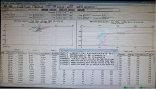
Data measured by vmadcps are recorded via the vessel-mounted Data Acquisition System (VmDas) software installed on two PCs in the main laboratory.  The recording is stopped everyday for the software to make a copy of the recorded data onto the ship server for daily processing. Every time the software is restarted, a new sequence will be created as a tracker on this routine event. All the operations and commands made on the PCs in main lab will be sent the deck unit of the vmadcp system. These boxes then send signals to the transducer to execute the commands from the PC terminals. The top one is for the 75 kHz instrument and middle one is for 150 kHz, the bottom one is a backup for 75 kHz.

A typical view of the screen of the PCs controlling the ADCP measurements

The measurements from vmadcps when in deep water are calibrated during processing from the bottom track data collected during shallow water transits. Bottom track is basically to measure the heading (position) and speed of the centre of the ship as measured by the ADCP when referenced to the sea floor. It provides the correction estimates on the amplitude and angle for the vmadcp measurements when the bottom cannot be “seen” within the range of the instrument.  Constrained by the maximum bottom track range, bottom track mode can only be working functionally in shallow waters (within the maximum range and also depending on the setup for each instrument).  

The ADCP deck units

 

Apart from the vessel-mounted ADCPs, we also deployed one moored-version ADCP with one of our moorings at the normal offshore extent of the Deep Western Boundary Current (WB4) to collect currents data above the mooring which otherwise would be missing when the mooring is knocked down in strong currents. Two more are deployed at the continental shelf-edge (WBADCP) to measure the currents inshore of WB1.

A self logging version of an ADCP being prepared for deployment before being mounted in a float

Discovery Friday (Captain Scott's Discovery)

As I write this final instalment of Discovery Friday, we are hove to, waiting for weather to pass to finish our work on the RAPID moorings. The waiting is frustrating but should only be an extra few days—nothing in comparison to the original RRS Discovery, which spent an extra year trapped in ice in Antarctica waiting to be free. 

Captain Scott built his ship from donations to the Antarctic expedition. It was the last wooden ship built in Britain, built by the Dundee Shipbuilder’s Company and launched in 1901. Discovery was built for life in the ice of Antarctica. She had a flat bottomed hull and bow designed to ride up over the ice to break it with pressure. She had a steam engine but relied heavily on sail power to provide sufficient propulsion. The propeller and rudder could be hauled out of the water to avoid damage. Built for the ice, she handled badly in open water and was prone to large rolls.

Scott and his crew set sail in August 1901 and sighted Antarctica in January 1902. They spent a month mapping the coastline before anchoring in McMurdo Sound. They would stay there, trapped in the ice for two years. The idea of being confined in a 50 metre long vessel for two years, trapped in ice, with 47 men would not be something I can imagine enjoying.

The expedition was a success remapping the location of the magnetic South Pole and achieving a record furthest south point of 82º 18’. The ship broke free of the ice in February 1904 and arrived back to the UK in September. The expedition was a success.

The ship took part in various roles for the next 20 years before returning to research and exploration in 1923. It was at this point she was christened a Royal Research Ship, really beginning the lineage that our current ship continues today.

Much like Discovery II would do, this original RRS Discovery spent much of her time in the Antarctic mapping whale populations. This formed part of the Discovery Investigations from which started the Discovery Collections, samples from which are still being used for scientific research to this day.

There are a number of photos and paintings of this old ship on the new RRS Discovery, including two nice watercolours in the conference room. My favourite, however, is in the mess, taken from Discovery’s time as a research vessel rather than her more famous time as Scott’s Antarctic exploration vessel. It shows two men taking sampling with nets over the side. They are clad in gear that you might expect more to be wore by someone on safari in the early 20^th Century. Perhaps these were the precursors of the hard hats and safety footwear we wear today. It is a nice picture to finish on as it completes the lineage of scientific research from the original Discovery through to our current home.

Written by Gerard (posted by Darren - slightly late due to a slow connection!)